DEBT LIMIT

Prolonged Negotiations Increase Taxpayer Costs and Disrupt Financial Markets

Report to Congress

March 2026

GAO-26-107872

United States Government Accountability Office

A report to Congress.

For more information, contact: Michael E. Clements at clementsm@gao.gov, Michael Hoffman at hoffmanme@gao.gov, or James R. McTigue Jr. at mctiguej@gao.gov.

What GAO Found

Debt limit impasses impose avoidable costs. As a projected date nears when the U.S. will be unable to meet all its financial obligations—the X date—investors often demand higher yields on new Treasury securities maturing near that date to compensate for the added risk. This increases the government’s borrowing costs.   GAO estimates that Treasury securities issued during periods of acute market concern over impasses between 2011 and 2023—the most recent impasses with complete data available at the time of GAO’s analysis—incurred a total of roughly $107 million to $161 million in increased immediate borrowing costs (in 2024 dollars), depending on the measure used to estimate market concern. Impasses also impose additional, hard-to-quantify costs, including long-term costs from reduced investor confidence in the Treasury market.

Note: For each impasse, GAO used two distinct measures of market concern to estimate increased borrowing costs. For more details, see fig. 2 in GAO-26-107872.

Debt limit impasses have also reduced the market value of outstanding Treasury securities. Market participants avoided securities maturing near a projected X-date, as those maturing after this date would be the first to default if the impasse were not resolved in time. GAO’s analysis found that these securities lost value relative to comparable ones maturing just before the X-date.

Impasse disruptions to Treasury markets can spread to short-term funding markets and funds closely tied to Treasury securities. In 2011 and 2013, such disruptions included higher borrowing rates and money market fund outflows. These disruptions prompted market participant actions to limit risk and manage future impasse effects. However, other disruptions can occur after impasses are resolved, as fluctuations in the Department of the Treasury’s cash balance create volatility in some markets.

GAO’s prior work has identified longstanding concerns about the debt limit (GAO-25-107089). The current debt limit process creates an unnecessary risk of U.S. default, with potentially devastating consequences for individuals, financial institutions, and the broader economy. The costs and market disruptions documented in this report further underscore the need for debt limit reform.   

Why GAO Did This Study

Congress imposes a legal limit on federal borrowing, known as the debt limit. Under the current process, Congress can approve spending increases or tax cuts without also ensuring that Treasury has sufficient borrowing authority to finance these decisions. In recent years, when the federal government has approached the debt limit, prolonged congressional negotiations on increasing or suspending the limit have repeatedly brought it close to being unable to continue paying obligations stemming from past spending and revenue decisions. If Treasury exhausts its borrowing authority and runs out of cash, a default will occur.

In this report, GAO examines how debt limit impasses—where outstanding debt reached the limit and Congress did not immediately raise or suspend it—between 2011 and 2023 affected Treasury’s borrowing costs and U.S. financial markets more broadly.

GAO analyzed financial market data and developed a suite of econometric models to estimate increased borrowing costs attributable to these impasses. GAO also reviewed relevant research, documentation, and laws. In addition, GAO interviewed agency officials and 17 financial market participants, selected to reflect a range of institution types and sizes.

What GAO Recommends

GAO previously outlined alternatives to the current debt limit process and recommended that Congress replace it with an approach that links debt decisions to spending and revenue decisions at the time they are made (GAO-15-476 and GAO-25-107089). GAO maintains that it is imperative that Congress take this action to prevent the recurring adverse effects of debt limit impasses.

 

 

 

Abbreviations
CMT	Constant Maturity Treasury
Federal Reserve	Board of Governors of the Federal Reserve System
LIBOR	London Inter-Bank Offered Rate
SOFR	Secured Overnight Financing Rate
TGA	Treasury General Account

 

 

March 25, 2026

Report to Congress

Congress imposes a legal limit on federal borrowing, known as the debt limit. The current debt limit process allows Congress to increase spending or decrease taxes without providing the Department of the Treasury sufficient borrowing authority to finance these decisions. In recent years, when the federal government has approached the debt limit, prolonged congressional negotiations on increasing or suspending the limit have repeatedly brought it close to being unable to continue paying obligations stemming from past spending and revenue decisions. If Treasury exhausts its borrowing authority and runs out of cash to continue paying government obligations, a default will occur.

Our existing body of work has demonstrated that these repeated impasses—where outstanding debt reached the debt limit and Congress did not immediately raise or suspend the limit—pose substantial risks for the nation. The consequences of a default could be devastating for individuals, financial institutions, and the economy. A default has the potential to disrupt financial markets; destabilize the economy; challenge financial regulators’ effectiveness in maintaining financial stability, including protecting depositors; weaken the dollar’s global use; and undermine the safety of Treasury securities, worsening the nation’s long-term fiscal path. Even without default, the current debt limit process has adverse effects. These include reduced investor confidence in Treasury securities used to finance government obligations and reputational harm to the nation, as reflected in downgrades to its sovereign credit rating.[1]

We also previously quantified the effect of early impasses on Treasury’s borrowing costs and the financial markets. For example, in 2015 we examined the 2013 debt limit impasse and found that it cost taxpayers tens of millions of dollars in increased borrowing costs—undermining the goal of financing the government at the lowest cost over time—and disrupted broader financial markets.[2] Since then, nine additional debt limit impasses have occurred, raising the question of their cumulative effect on the nation.

We prepared this report at the initiative of the Comptroller General. It is part of our continuing efforts to help Congress address challenges related to the debt limit. This report examines how debt limit impasses between 2011 and 2023—the most recent impasses with complete data available at the time of our analysis—affected Treasury’s borrowing costs and the U.S. financial markets more broadly.

To address this objective, we conducted multiple quantitative analyses in the following areas:

·         Treasury’s borrowing costs. We conducted econometric modeling to estimate the immediate effect of delays in raising the debt limit on the Department of the Treasury’s borrowing costs during impasses between 2011 and 2023.[3] See appendix I for details on this methodology and its limitations and appendix II for regression results.

·         Disruptions in the secondary market for Treasury securities. We analyzed data from 2011 through 2023 on yields in the Treasury secondary market—where previously issued Treasury securities are traded among public and private parties—to assess how debt limit impasses have affected this market. To estimate the change in value of securities maturing on or just after a projected X-date—the date when the U.S. government would no longer be able to meet all its financial obligations—we calculated the difference between the peak yield and the yield observed when acute market concern over the impasse first became evident.[4] We then compared this difference with the effective federal funds rate at that same point in time.

·         Value of at-risk Treasury securities. We used data—including Treasury’s Monthly Statement of Public Debt—from 2011 through 2023 to calculate the amount of principal and interest due on Treasury securities during the month following a projected X-date and their outstanding face value.

·         Treasury General Account (TGA) balance fluctuations. We used publicly available Federal Reserve Bank of St. Louis data on the TGA, which Treasury uses to pay government obligations, to assess changes in balances during and after the 2023 debt limit impasse.

For these quantitative analyses, we assessed the reliability of the underlying data by reviewing related documentation and testing for missing data, outliers, and obvious errors. We determined the data to be sufficiently reliable for the purposes described above.

In addition, we reviewed relevant research and documentation from Treasury, including its Office of Financial Research, and from the Federal Reserve System, including the Board of Governors, the Federal Open Market Committee, and the regional Reserve Banks.[5] We also reviewed related research published by academics, the International Monetary Fund, the Congressional Research Service, and the Congressional Budget Office, as well as our prior related work.[6]

We analyzed Treasury documents and relevant laws from January 2011 through June 2023—the period covering the debt-limit impasses examined in this report—to identify dates when the U.S. reached the debt limit and the limit was raised or suspended. We also identified the estimated dates when the government would exhaust its cash, borrowing authority, or available extraordinary measures to continue to make payments for Treasury debt and other obligations.

We interviewed staff from Treasury and the Board of Governors of the Federal Reserve System (Federal Reserve). We also interviewed representatives of 17 financial market participants, representing primary dealers, banks, money market funds, clearing banks, a hedge fund, and data processing vendors.[7] We selected these participants to reflect a range of institution types, sizes (measured by total assets), and participation in the Treasury market, including holdings of Treasury securities. The views expressed in these interviews are not generalizable to all market participants or observers. To characterize interviewee responses in this report, “some” refers to three to five interviewees, “several” refers to more than five but less than half, and “most” refers to more than half of the interviewees.

We conducted this performance audit from November 2024 to February 2026 in accordance with generally accepted government auditing standards. Those standards require that we plan and perform the audit to obtain sufficient, appropriate evidence to provide a reasonable basis for our findings and conclusions based on our audit objectives. We believe that the evidence obtained provides a reasonable basis for our findings and conclusions based on our audit objectives.

Background

Financing the Federal Government

Treasury Securities Treasury securities include bills, notes, and bonds. ·       Bills. Short-term securities maturing in 1 year or less. Currently issued regularly in 4-, 6-, 8-, 13-, 17-, 26-, and 52-week maturities. ·       Notes. Interest-bearing securities with a fixed maturity of no less than 1 year and no more than 10 years from their issue date. Currently issued in 2-, 3-, 5-, 7-, and 10-year maturities. ·       Bonds. Interest-bearing securities with maturities over 10 years. Currently issued in 20- and 30-year maturities. Source: GAO. | GAO‑26‑107872

When the federal government runs a budget deficit (i.e., spending exceeds revenue), Treasury borrows additional funds by issuing Treasury securities (see sidebar). These funds are largely raised through regular auctions, known as the primary market, where marketable Treasury securities are sold. Eligible bidders include individuals, primary dealers, other brokers and dealers, various investment funds, banks, and international entities, among others.

Once the auctioned Treasury securities are issued to successful bidders, they enter the secondary market, where they are traded among public and private parties. Yields—or interest rates—at auction generally closely track yields of previously issued Treasury securities trading in the secondary market.

Treasury’s primary debt management goal is to finance the government’s borrowing needs at the lowest cost over time. The government’s cost of borrowing is largely determined by the volume of each type of marketable Treasury security and its yield when issued. The interest cost depends on a variety of factors, including investor demand, federal fiscal policy, and monetary policy.

Treasury securities have three key characteristics that have made them highly attractive to a wide range of investors (see fig. 1).

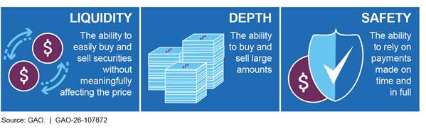
Treasury securities are held by a wide variety of public and private investors in the U.S. and abroad, including hedge funds, money market funds, mutual funds, banking institutions, and foreign central banks.[8] Investors hold Treasury securities for a variety of reasons, including cash and liquidity management, collateral, hedging, and as long-term investments. For example, financial institutions and corporate treasurers often treat Treasury securities as a close substitute for cash. They are also one of the least expensive and most widely used forms of collateral for financial transactions. In addition, Treasury securities serve as a benchmark for pricing many other financial products, such as corporate bonds, derivatives, and mortgages.

Treasury General Account

Treasury maintains an operating balance in the Treasury General Account (TGA), which is equivalent to a checking account for the federal government. The account is maintained at the Federal Reserve Bank of New York.[9] The TGA makes payments for government obligations, including payments on outstanding debt, and receives deposits of taxes, customs duties, public debt receipts, and proceeds from the sale of Treasury securities.

The TGA balance fluctuates daily, due in part to Treasury’s varying needs week-to-week. To ensure that Treasury can continually fund government obligations, it has a standing policy to maintain a TGA balance equivalent to approximately 1 week of outflows, subject to a minimum TGA balance of roughly $150 billion.[10] The TGA balance has averaged approximately $800 billion outside of debt limit impasses in recent years.

Debt Limit

Congress first passed statutory limits on federal debt during World War I. This action was taken to eliminate the need for Congress to approve each new debt issuance and to provide Treasury with greater flexibility in how it finances the government’s day-to-day borrowing needs.

Federal debt subject to the limit consists of two categories:

·         Debt held by the public refers to Treasury-issued securities, including bills, notes, and bonds.

·         Debt held by the government refers to debt held in government accounts consisting of investments in special Treasury securities made by government trust funds, such as those for Social Security, civil service retirement, and Medicare, as well as the Federal Deposit Insurance Corporation’s Deposit Insurance Fund and the Department of Labor’s Unemployment Trust Fund.

The statutory debt limit set by Congress caps the total amount of federal debt that can be outstanding at a given time. It does not control the amount of government spending but instead limits Treasury’s authority to finance spending and revenue decisions that Congress has already made. Borrowing enables Treasury to meet existing, legally committed obligations, such as Social Security and Medicare benefits, military salaries, interest on the national debt, and tax refunds. Raising the debt limit does not authorize new spending.

Debt Limit Impasses and Extraordinary Measures

A debt limit impasse is generally understood to start when outstanding debt reaches the statutory limit and continues until Congress passes legislation to raise or suspend the limit. Between 2011 and 2025, 13 impasses took place; each impasse ended through temporary suspensions of or increases to the debt limit.[11]

During debt limit impasses, Treasury manages both the level of cash on hand and borrowing to avoid exceeding the debt limit. To continue paying government obligations, including payments on outstanding debt, Treasury can draw down the TGA balance and continue to make payments as they come due. Treasury also can invoke “extraordinary measures”—temporary actions that either reduce the amount of outstanding debt subject to the limit or suspend or postpone certain increases in debt subject to the limit. For example, Treasury can suspend investment of federal employee retirement contributions in the Thrift Savings Plan’s Government Securities Investment Fund (G Fund).

X-Date and Default

When the outstanding debt is near or at the statutory limit, Treasury typically estimates a date or date range for when the government will no longer have sufficient cash, borrowing authority, or available extraordinary measures to make timely payments on Treasury debt or other federal obligations. This date is commonly referred to as the X-date. For the purposes of this report, the U.S. would be considered in default if it reached the X-date and did not make timely payments on Treasury debt obligations. A default also would hinder the government’s ability to make nondebt payments, such as for program benefits, contractual services and supplies, and federal employee salaries.

Short-Term Funding Markets and Money Market Funds

Short-term funding markets—such as repurchase agreements and commercial paper—and money market funds enable financial institutions to borrow and lend cash and help underpin the functioning of the financial system. Financial institutions and corporations rely on cash borrowing through these markets and funds to support many routine financial transactions. As detailed in table 1, Treasury securities play a central role in these markets and funds.

	Description
Repurchase agreements	A repurchase agreement, or repo, is a financial transaction in which an institution sells a security to an investor and commits to repurchasing the security later at a higher price. In practice, the transaction functions as a collateralized loan, where the difference between the initial sale price and the repurchase price represents the interest paid. Repos often use Treasury securities as collateral. The repo market is critical to the health and stability of U.S. financial markets and the broader economy because it serves as an important source of short-term funding for market participants. According to the Board of Governors of the Federal Reserve System, the U.S. repo market is one of the world’s most important financial markets, with a gross size of $11.9 trillion in 2024. Cash lenders—typically money market funds or financial institutions such as banks—use repos to earn a return on their cash while receiving collateral as protection against loss of principal in the event of default. Cash borrowers—typically hedge funds or broker-dealers—use repos to finance their holdings of securities or to obtain leverage.
Commercial paper	Commercial paper is unsecured, short-term debt issued by nonfinancial corporations, banks, and other financial institutions. It provides a flexible way to fund institutions and manage working capital. Institutional investors participating in this market include investment companies, retirement accounts, state and local governments, and financial and nonfinancial firms. Treasury securities often serve as a benchmark against which investors compare the returns on other products, such as commercial paper. As of the end of 2024, approximately $1.2 trillion in commercial paper was outstanding.
Money market funds	Money market funds are mutual funds that invest in high-quality, short-term debt securities and pay dividends that generally reflect short-term interest rates. These funds serve as intermediaries in the short-term funding markets, linking investors with cash to lend and borrowers with short-term funding needs. As of 2024, they held approximately $7 trillion in total assets. Money market funds invest in securities that underlie the short-term funding markets, such as short-term U.S. Treasury securities, short-term municipal securities, and commercial paper. They offer investors generally safe, liquid, and short-term investments, while providing borrowers to access low-cost funds. They also provide important financing to governments, banks, and nonfinancial corporations. As a result, their orderly functioning is essential to the performance of broader financial markets and the U.S. economy. Although money market funds, like checking accounts, offer investors interest and can be easily converted to cash, the funds are not insured by the Federal Deposit Insurance Corporation or other federal insurance programs. As a result, if these funds are perceived to be at risk, they may be vulnerable to investor runs. As of March 2025, money market funds held approximately 36 percent of outstanding Treasury bills.

Source: GAO. | GAO‑26‑107872

Alternatives to the Current Debt Limit Process

We have made recommendations to Congress on the debt limit in previous reports. Specifically, in 2015, we recommended that Congress consider adopting an approach to limit debt that both (1) minimizes disruptions to Treasury and financial markets and (2) better links decisions about the debt limit with decisions about spending and revenue at the time those decisions are made.[12]

We also identified three alternatives to the current debt limit process, each of which meets these criteria while maintaining congressional control and oversight over federal borrowing:

·         Alternative 1: Link action on the debt limit to the budget resolution.

·         Alternative 2: Provide the administration with the authority to increase the debt limit, subject to a congressional motion of disapproval.

·         Alternative 3: Delegate broad authority to the administration to borrow as necessary to finance laws passed by Congress.

As of January 2026, Congress had not yet addressed our 2015 recommendation that it consider alternative approaches to the current debt limit process.

In 2024, after highlighting the potential consequences of U.S. default, we recommended that Congress consider immediately removing the debt limit and adopting an approach that better links decisions about the debt with decisions about spending and revenue at the time those decisions are made.[13] As of January 2026, Congress had also not yet addressed this recommendation.

Eliminating the current debt limit process would not prevent Congress from enacting policies that improve the sustainability of the nation’s fiscal path. In previous work, for example, we reported that fiscal rules and targets can help manage debt by controlling spending and revenue.[14]

Repeated Debt Limit Impasses Have Raised Borrowing Costs and Disrupted Financial Markets

Debt limit impasses impose avoidable costs on the nation. As a projected X-date nears, investors often demand higher yields at auctions for new Treasury securities to compensate for the increased risk of delayed payment. These higher yields ultimately increase Treasury’s borrowing costs—an unnecessary expense borne by taxpayers. Impasses also disrupt the secondary market for Treasury securities, where previously issued debt can be traded among public and private parties. These disruptions can spread to other short-term funding markets critical to the broader economy. Our prior work has identified serious and longstanding concerns about the debt limit and the potentially devastating consequences default can pose for individuals, financial institutions, and the economy. The costs and financial market disruptions documented in this report further underscore the need for debt limit reform.

Impasses Generally Increased Borrowing Costs for the U.S. Government and Taxpayers

Debt limit impasses impose avoidable costs on the U.S. government and, ultimately, taxpayers. These costs run counter to Treasury’s goal of financing the government at the lowest cost over time. In the days and weeks leading up to a projected X-date—the date when the nation would no longer be able to meet all its financial obligations—auctions for new Treasury securities can reflect acute market concern. That is, investors may fear potential disruptions or delays in debt payments and the ensuing economic volatility. When investors demand compensation for this added risk and uncertainty in the form of higher yields (i.e., lower prices at auction) on newly issued securities, that compensation is ultimately borne by taxpayers in the form of increased interest payments.

We estimated the immediate effect of debt limit impasses on Treasury’s borrowing costs through econometric modeling. We included eight debt limit impasses that occurred between 2011 and 2023 in our analysis.[15] Specifically, we estimated (1) the change in yields on securities auctioned by Treasury during the periods of acute market concern over each impasse and (2) the associated immediate increase in interest costs (i.e., those incurred within the first year of the auctions).[16]

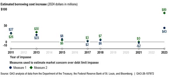
Overall, we found that Treasury securities issued during periods of acute market concern over the eight impasses incurred a total of roughly $107 million to $161 million in increased borrowing costs (in 2024 dollars) during the first year following issuance. This range reflects two distinct measures we used to estimate market concern over the debt limit, each with different analytical advantages (see fig. 2 for cost estimates corresponding to each individual impasse).[17]

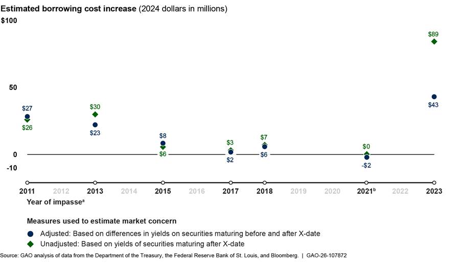
Note: Estimates are based on GAO econometric models assessing the effect of delays in raising the debt limit on the Department of the Treasury’s borrowing costs. The estimates focus on Treasury securities that (1) were issued during periods of acute market concern over eight debt limit impasses between 2011 and 2023 and (2) were set to mature on or after the projected X-date for those impasses—the date when the U.S. government would no longer be able to meet all its financial obligations. The estimates reflect borrowing costs incurred during the first year following the securities’ issuance. See app. I of GAO‑26‑107872 for methodology details and limitations and app. II for in-depth regression results.

^aImpasses in 2013, 2014, and 2019 were excluded because their periods of acute market concern were too brief for estimation purposes. A 2012 impasse was excluded because it involved an automatic statutory increase and thus no cause for market reaction.

^bTwo consecutive 2021 impasses are combined: the first ended in October with a $480 billion debt limit increase and the second in December with a $2.5 trillion increase.

For all but the 2021 impasses we modeled, we found that market concern over the debt limit was associated with immediate costs to Treasury and therefore taxpayers. Those costs were largely concentrated in bills (which have shorter maturities), though affected maturities varied by impasse. We did not find observable, immediate costs associated with the impasses that occurred in 2021. This may reflect the unusual context of that time, including the two consecutive impasses that occurred that year. Moreover, the federal government’s large-scale COVID-19 response and the related strong demand for safe assets, such as Treasury securities, may have dampened investors’ perception of risk and reduced their reluctance to hold securities exposed to potential default.[18]

Our estimates focus on Treasury securities issued during periods of acute market concern over each impasse, and they reflect costs incurred during the first year following the securities’ issuance. The extent of market concern varied across impasses and likely reflected investors’ assessment of political risk and how quickly the impasse would be resolved. In addition to the risk premium demanded at each auction of affected securities, total costs depended on both the number of affected auctions during the period and the size of each offering.

Beyond the costs captured in our model, debt limit impasses impose additional costs on taxpayers that we did not seek to quantify, given the challenges of doing so with reasonable confidence. For example, there may be persistent costs from reduced investor confidence in the safety and liquidity of the Treasury market. While small on a per-auction basis, these costs could persist at auctions held long after an impasse is resolved. One market participant we interviewed noted that additional taxpayer costs likely arise from the rapid issuance of bills after an impasse resolution, not because of fears over their creditworthiness but due to the sheer volume of supply.

Moreover, as we have previously reported, Treasury incurs administrative costs—ultimately borne by taxpayers—when managing impasses. These include the implementation and oversight of extraordinary measures to continue meeting the government’s obligations.[19]

There are also limitations to our multivariate regression models’ ability to measure changes in Treasury’s borrowing costs attributable to debt limit impasses. Our models controlled for multiple factors that affect Treasury rates. However, various unobserved factors could increase or decrease our estimates.[20] See appendix I for detailed information on our estimation methodology and its limitations and appendix II for in-depth regression results.

Impasses Reduced the Value of At-Risk Treasury Securities in the Secondary Market

Debt limit impasses have repeatedly disrupted the secondary market for Treasury securities—the market in which previously issued Treasury securities are bought and sold among investors. These disruptions were driven by many investors avoiding “at-risk” Treasury securities—those maturing on or soon after the projected X-date—given fears of potential default. As demand for these securities declined, their market value fell. Market participants also reported that, in some cases, liquidity also decreased as fewer types of investors were willing to purchase them from investors looking to shed such holdings.

Market Participants Minimized Their Exposure to At-Risk Treasury Securities

The dollar value of Treasury securities considered to be at-risk and therefore avoided by market participants was substantial. As figure 3 shows, during impasses from 2011 through 2023, the outstanding value of securities that matured or paid out interest on a projected X-date or in the subsequent month ranged from $1.3 trillion to $5.9 trillion—representing 9 to 26 percent of total debt held by the public.

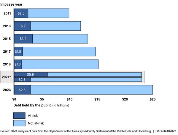
Note: For purposes of this analysis, we defined at-risk Treasury securities as those that matured or paid out interest on an impasse’s projected X-date or in the subsequent month. The projected X-date is the date when the U.S. government would be unable to continue meeting all its obligations. The amounts displayed above reflect the outstanding face value of these securities. Impasses in 2013, 2014, and 2019 were excluded because their periods of acute market concern over the debt limit were too brief for estimation purposes. A 2012 impasse was excluded because it involved an automatic statutory increase and thus no cause for market reaction.

^aTwo consecutive impasses occurred in 2021: the first ended in October with a $480 billion debt limit increase and the second in December with a $2.5 trillion increase.

Most market participants we spoke with said they actively avoided Treasury securities maturing around a projected X-date.[21] This avoidance included selling these securities, not purchasing them, and not accepting them as collateral. Some market participants went further, avoiding all Treasury securities maturing several months before and after projected X-dates to minimize the risk of holding securities at risk of delayed payment or default. Those that continued to buy these securities received higher yields to compensate for higher risk.

Further, some market participants said they also avoided notes and bonds with coupon payments—semiannual interest payments—expected around the projected X-date due to uncertainty about whether those payments would be made in the event of a default. Representatives of one dealer said that during the 2023 impasse, they sold all notes and bonds with coupon payments near the projected X-date, citing significant cash flow risks.

Market participants who actively avoided securities maturing around the X-date cited multiple reasons for doing so. Some expressed concerns that in the event of default, the market would not be able to transact in defaulted securities beyond their original maturity date, and investors might not receive timely payment on maturing securities.[22] Others noted that avoiding such securities was important to reassure clients and uphold their reputations as prudent counterparties.

Several market participants identified money market funds as being especially sensitive to holding at-risk Treasury securities and likely to minimize their exposure more than other participants. Money market funds are vulnerable to unexpected redemptions if investors perceive a risk of losses.[23] Excess exposure to at-risk Treasury securities that rapidly decline in value can undermine funds’ perceived stability. As a result, money market funds may proactively avoid or sell such securities to reassure investors.

Representatives of the two money market funds we spoke with sold at-risk Treasury securities, and one avoided purchasing all Treasury securities set to mature within several months of a projected X-date. They both told us it was preferable to invest cash in other assets, such as agency securities, or with the Federal Reserve via its Overnight Reverse Repurchase Agreement Facility rather than hold securities maturing near a projected X-date.[24]

However, avoiding at-risk Treasury securities created challenges for fund managers seeking to maintain their investment strategies. Representatives of one fund explained that balancing the need to mitigate impasse risks with the requirement to comply with money market fund regulations was particularly difficult for products whose core investment strategy is to invest primarily in Treasury securities.[25] Representatives of another fund stated that, during the 2023 impasse, avoiding at-risk securities lengthened the fund’s weighted average maturity. This shift occurred as the Federal Reserve was raising rates, which heightened the fund’s interest rate risk and drove a noticeable decline in the market-based valuation of its holdings—although the fund ultimately did not need to adjust its share price.[26]

Nevertheless, some other market participants have been willing to purchase Treasury securities during an impasse. Representatives of one dealer noted that they would purchase at-risk securities if valuations became sufficiently attractive, but that they generally sought to limit exposure since these securities tend to lose value ahead of most X-dates. Some also noted that hedge funds, state and local governments, and foreign central banks have been among the entities willing to purchase these securities. They noted that such buyers may be more tolerant of additional risk in exchange for higher yields and may expect that an impasse would resolve before the X-date.[27]

At-Risk Treasury Securities Were Sometimes Harder to Trade During Impasses

Most market participants we spoke with observed decreased liquidity—the cost and ease of exchanging assets for cash at needed volumes—for at-risk Treasury securities during past impasses.[28] Decreased liquidity can raise costs for Treasury holders that need to sell during an impasse and, in extreme cases, may prevent them from selling at all. One money market fund representative described how, during the 2023 impasse, some at-risk Treasury securities were traded only “by appointment,” meaning dealers would arrange a sale for a client but were unwilling to buy and hold the securities themselves. This arrangement indicates that dealers were not confident there would be sufficient buyer interest for the at-risk securities.

At-Risk Treasury Securities Lost Value as X-Dates Approached

As each projected X-date approached, Treasury market activity reflected increasing concern about the risk of default on at-risk Treasury securities. Several market participants we interviewed said they either shared these concerns or observed them among clients or peer institutions. Acute market concern became evident when yields on individual Treasury bills with similar maturities started to diverge, depending on whether a given bill’s maturity date fell immediately before or after the projected X-date. Under normal conditions, these securities would be priced almost identically in the secondary market, as they share the same issuer and nearly identical maturities, and therefore present essentially the same interest rate risk.[29]

However, our analysis found these prices—and therefore yields—diverged during the impasses between 2011 and 2023. Yields spiked for Treasury securities maturing immediately after the projected X-date—those perceived to be at risk—relative to those that matured just before, which were not perceived to be a default risk. As shown in figure 4, this divergence is observable to varying degrees across most recent impasses.

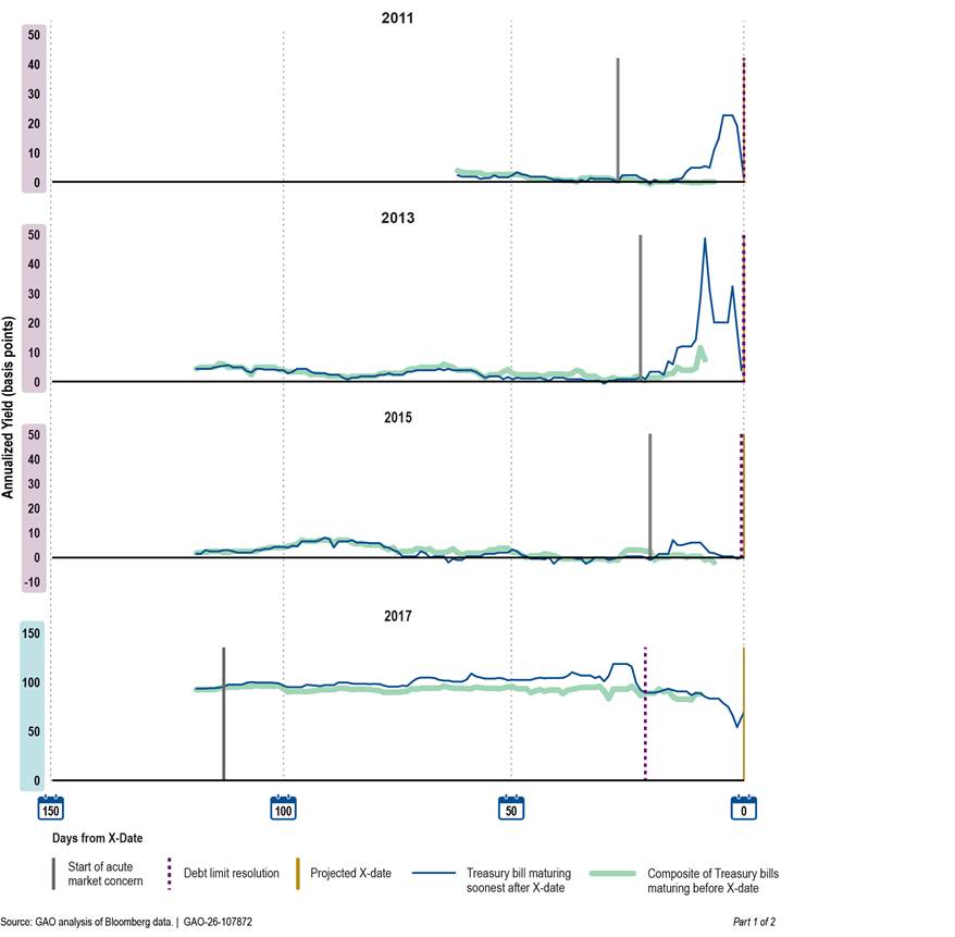
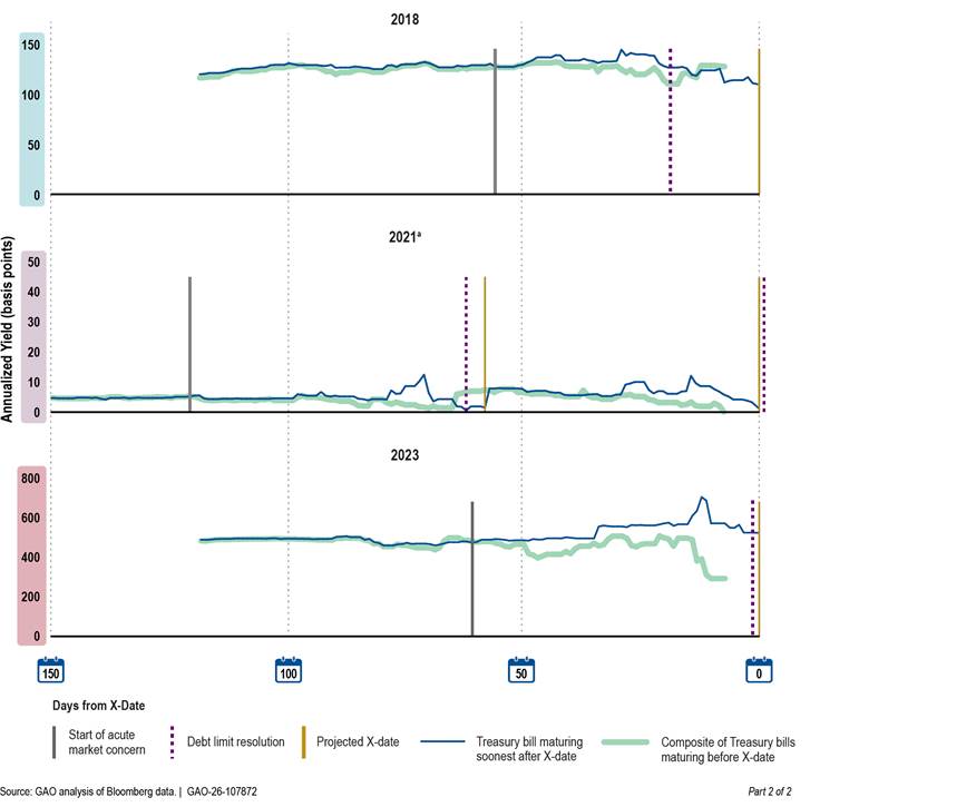
Note: We identify the start of acute market concern as the point when yields on Treasury bills maturing just after the projected X-date—the date when the U.S. government would be unable to continue meeting all its obligations—start to persistently exceed those of bills maturing just before the X-date. Impasses in 2013, 2014, and 2019 were excluded because their periods of acute market concern over the debt limit were too brief for estimation purposes. A 2012 impasse was excluded because it involved an automatic statutory increase and thus no cause for market reaction.

^aTwo consecutive 2021 impasses are combined: the first ended in October with a $480 billion debt limit increase and the second in December with a $2.5 trillion increase.

The yield spikes represent a drop in the value of the at-risk Treasury securities in the portfolios of their holders. Some market participants told us that the significance of these spikes during impasses depended on broader market conditions, including the prevailing interest rate. As a share of the effective federal funds rate—a measure of the prevailing short-term interest rate—the two earliest impasses (2011 and 2013) caused the largest relative yield distortions.[30] Yields on at-risk securities spiked to over three times the federal funds rate in 2011, and over five times the rate in 2013 (see fig. 5).

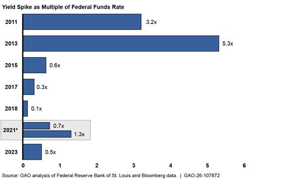
Note: For purposes of this analysis, we defined an at-risk Treasury security as either one that matured on the projected X-date or, if no Treasury security matured on the X-date in a particular impasse, the security that matured soonest after that date. The projected X-date is the date when the U.S. government would be unable to continue meeting all its obligations. Impasses in 2013, 2014, and 2019 were excluded because their periods of acute market concern over the debt limit were too brief for estimation purposes. A 2012 impasse was excluded because it involved an automatic statutory increase and thus no cause for market reaction.

^aTwo consecutive impasses occurred in 2021: the first ended in October with a $480 billion debt limit increase and the second in December with a $2.5 trillion increase.

Some market participants stated that spikes in secondary market yields of at-risk Treasury securities during past impasses resulted in realized losses as they were forced to sell them under unfavorable market conditions. These spikes also resulted in adverse effects in other markets due to the central role Treasury securities play in global finance. For example, one market participant told us that when the value of at-risk securities declines, some market participants request that clients swap out at-risk securities collateralizing existing financial agreements.

Impasses in 2011 and 2013 Disrupted Short-Term Funding Markets and Funds, Prompting Adjustments by Market Participants

When impasses disrupt Treasury markets, the disruptions can spread to short-term funding markets and funds closely tied to the Treasury securities market. These disruptions were seen during the 2011 and 2013 impasses, affecting repo markets and money market funds, for example, and prompting market participants to take protective measures to manage impasse-related effects. The effects of disruptions were less evident in the more recent impasses we analyzed. However, other disruptions can occur after impasses are resolved, as fluctuations in Treasury’s cash balance create volatility in some markets.

Impasses Have Disrupted Multiple Short-Term Funding Markets and Funds

Short-term funding markets and funds that have been disrupted by previous impasses include the repurchase and commercial paper markets and money market funds.

Repurchase Agreement Market

During the 2011 and 2013 impasses, the repo market experienced disruptions in the form of higher rates. For example, some market participants said repo rates rose during both impasses, with one citing increased rates in the 2011 impasse by approximately 20 to 30 basis points.[31] In addition, the Federal Reserve noted that repo rates increased in 2013 by 10 to 18 basis points. Higher or more volatile repo rates make short-term borrowing more expensive and funding sources less reliable during the period of increased volatility.

In 2015, we reported that yields on overnight repo agreements—those that last only 1 day—increased during the 2013 impasse from 4.5 basis points to as high as 23 basis points in the weeks leading up to the X-date, an increase of more than 500 percent.[32]

Commercial Paper Market

We previously reported that debt limit impasses likely affected other short-term markets, such as the market for commercial paper—short-term securities issued by corporations to raise cash needed for current transactions.[33] Because Treasury securities often serve as a benchmark for comparing the returns of other products, increased rates on Treasury securities can lead to increased rates in other markets, such as commercial paper, affecting borrowing costs for a range of borrowers. For example, during the 2013 debt limit impasse, the yield on 1-month commercial paper from financial institutions, such as banks, rose from 5 basis points to 21 basis points in the weeks leading up to the X-date. Yields also increased for other maturities and for commercial paper issued by nonfinancial issuers. In addition, we reported that during the 2013 impasse, some commercial paper issuers delayed or otherwise changed issuance plans, with the amount of commercial paper outstanding issued by financial institutions declining each week as the X-date approached.

Money Market Funds

Money market funds are among the market participants most vulnerable to impasses because their holdings are both highly reliant on Treasury securities and transparent to their investors, who can withdraw funds at will. If investors become worried about the soundness of their Treasury holdings, money market funds can be susceptible to runs.[34]

Moreover, empirical research and some market participants highlighted the risk of money market outflows during impasses. For example, two studies found evidence of investor outflows at some money market funds during the 2011 and 2013 impasses.[35] Some market participants we spoke with also highlighted the risk of impasses causing large, rapid outflows from money market funds. They said impasses make it challenging to manage holdings of Treasury securities. Investors may assess whether their funds have concentrated investments in at-risk Treasury securities and may start to withdraw money from the funds if they perceive this risk.

We previously reported that if shareholders perceive loss risk, they have an incentive to be the first to redeem their shares before prices fall.[36] To meet redemptions, a money market fund could use its cash and sell liquid securities to pay redeeming shareholders. However, it may also need to sell less liquid securities at a loss—potentially causing losses for remaining shareholders.

Market Participants Have Taken Steps to Protect Against Impasse-Related Disruptions

While short-term markets experienced disruptions during the 2011 and 2013 impasses, the effects of disruptions were less evident in the more recent impasses we analyzed. We found that market participants have taken steps to manage the impact of impasses by limiting their risk exposure. These actions have also helped reduce the risk of broader market disruptions caused by last-minute panic over a potential default.

Exclusion of At-Risk Treasury Securities from Collateral

Collateral helps reduce the risk of lending—and therefore the cost of borrowing—but collateral only protects the lender if it holds its value. As discussed above, at-risk Treasury securities do not fully hold their value during a debt limit impasse. We previously reported that market participants said they had established the ability to exclude individual Treasury securities from the types of collateral they would accept.[37] In doing so, they limited their exposure to at-risk Treasury securities in the repo market during an impasse.

In addition, some major repo market participants have permanently excluded all Treasury securities maturing the next business day from collateral they accept, which they identified as a change attributable to impasses. According to one U.S. clearing bank, this exclusion began on a client-by-client basis among parties to repo agreements during the 2011 impasse. By 2021, it had become a widely recognized contract term, when the Depository Trust and Clearing Corporation excluded next-day-maturing securities from the collateral accepted through central clearing operations.[38]

Some market participants told us that this change has raised their costs for holding next-day-maturing securities. This is because they may need to use higher-cost equity from their own balance sheets, rather than borrowing at lower rates in the repo market, to fund their holdings of excluded Treasury securities. While these costs may be small on an individual basis, they can accumulate across the large number of repo transactions that occur throughout financial markets.

Federal Reserve’s Overnight Reverse Repo Facility

As noted above, money market funds can be particularly affected by debt limit impasses and subject to runs if their investors worry about the soundness of their Treasury holdings. Access to the Federal Reserve Overnight Reverse Repo Facility can help mitigate this risk by allowing eligible money market funds to earn interest on risk-free investments in the facility, which has had a stabilizing effect on money market funds.[39] For example, one study found that funds accessing the facility experienced reduced fund outflows during the 2013 impasse compared with the 2011 impasse, when the facility was not yet available.[40]

Actions to Prepare for Impasses

Most market participants we spoke with reported taking steps to prepare for debt limit impasses that often require what they characterized as significant financial and personnel resources. Reported efforts included assessing potential impasse effects, rebalancing portfolios, and closely monitoring holdings—particularly those involving at-risk Treasury securities. Participants also reported developing and refining internal “playbooks” to guide their response in the event of a default and crafting strategies to mitigate potential risks. Several noted that repeated impasses, along with the need to respond to client concerns, imposed substantial direct costs and required them to spend time on impasses that could have been spent on other business functions.

Fluctuations in Treasury’s Cash Balance Can Also Disrupt Markets

In addition to disruptions to short-term funding markets during the 2011 and 2013 impasses, some market participants said impasses have disrupted repo markets when Treasury rebuilt the balance of the Treasury General Account (TGA). Rebuilding this account can reduce the amount of cash available in the financial system for trade in the repo market.

As we previously reported, debt limit impasses reduce Treasury’s cash balance, as limited borrowing authority leads it to use available cash to meet obligations.[41] This spending increases the amount of cash in the financial system. Once an impasse resolves, Treasury rebuilds its balance to normal levels by rapidly issuing debt (see fig. 6).

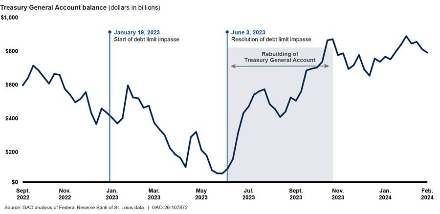
Rebuilding Treasury’s balance through debt issuance reduces the amount of cash in the financial system, which reduces the cash available to borrowers in the repo market. This occurs because payments for Treasury securities move from the banking system into the TGA. When cash in the financial system is already tight, this sudden drop can pose stability risks to institutions dependent on repo funding—potentially disrupting the broader financial system.[42] One study found that repo rates rise when impasses that deplete the TGA require Treasury to rebuild its balance.[43]

Impasses also pose an additional challenge for the Federal Reserve as it conducts monetary policy. For example, in early 2025, debt limit dynamics and changes in TGA balances were among the factors that prompted the Federal Open Market Committee to consider slowing the pace of its reduction of Treasury holdings, which reduces cash in the financial system. This reduction can make it more expensive for borrowers to obtain short-term funding. According to the Treasury Borrowing Advisory Committee, large changes in the TGA can cause fluctuations in the amount of cash in the financial system.[44] The committee stated that concerns about the 2025 debt limit likely prompted the Federal Reserve to temporarily slow monetary policy changes to avoid market disruptions associated with rebuilding the TGA—potentially before achieving its goal of reducing inflation.[45]

Debt Limit Reform Is Needed to Avert Unnecessary Costs and Disruptions

Our prior work on the federal debt limit has identified serious and long-standing concerns regarding the debt limit’s adverse consequences for the nation.[46] Chief among them is that the current debt limit process creates an unnecessary risk of U.S. default, with potentially devastating consequences for individuals, financial institutions, and the economy.[47]

This report further reinforces the need for reform. Our findings demonstrate that, even in the absence of default, the current debt limit process creates avoidable taxpayer costs and financial market disruptions.

To date, market participants have taken steps to mitigate the immediate financial market consequences of debt limit impasses by adjusting their portfolios and planning for impasse effects on Treasury markets. However, the resources expended to manage debt limit risk impose costs on the financial sector beyond those observable in Treasury auction pricing. Further, repeated impasses may weaken the attractiveness of Treasury securities and reduce the overall demand for U.S. debt.

We have previously recommended that Congress replace the debt limit with an approach that better links the debt level with decisions about spending and revenue at the time those decisions are made.[48] This would remove the risk of default by ensuring that all commitments of federal dollars are accounted for without the need for subsequent negotiations over the debt limit. Removing this risk would also prevent the financial market disruptions and costs to Treasury and market participants that result from recurring debt limit impasses.

In April 2025, the Treasury Borrowing Advisory Committee concurred that the debt limit has many known negative impacts with no clear benefit and concluded that the best option would be to eliminate it altogether.[49] However, as of January 2026, the debt limit remained in place and Congress had not yet implemented our recommendations for reform.

To avoid the risk of default—with its potentially devastating effects—and to prevent the recurring costs and disruptions associated with repeated impasses, we reiterate our recommendation that Congress consider replacing the debt limit with an effective alternative.

Agency Comments

We provided sections of a draft of this report to the Federal Reserve and Treasury for technical review. The agencies provided technical comments, which we incorporated as appropriate.

We are sending copies of this report to the appropriate congressional committees, the Chair of the Board of Governors of the Federal Reserve System, the Secretary of the Treasury, and other interested parties. In addition, the report is available at no charge on the GAO website at https://www.gao.gov.

If you or your staff have any questions about this report, please contact Michael E. Clements at clementsm@gao.gov, Michael Hoffman at hoffmanme@gao.gov, or James R. McTigue Jr. at mctiguej@gao.gov. Contact points for our Offices of Congressional Relations and Media Relations may be found on the last page of this report. GAO staff who made key contributions to this report are listed in appendix III.

Michael E. Clements
Director, Financial Markets and Community Investment

Michael Hoffman
Chief Economist, Applied Research and Methods

James R. McTigue, Jr.
Director, Strategic Issues

To estimate the immediate effect of delays in raising the debt limit on the Department of the Treasury’s borrowing costs for debt limit impasses between 2011 and 2023, we developed a suite of econometric models. For each impasse, we estimated two debt-limit-induced yield premiums across most maturities, excluding those for which estimates could not be reliably produced. This resulted in 119 time-series regressions that form the basis of our cost estimates. The models resulted in estimates of how interest rates on newly auctioned Treasury securities changed as a result of each impasse. We applied these estimates to Treasury auctions held during the relevant period to arrive at an estimate for the direct costs to Treasury from the debt limit impasse.

Our econometric models use time-series analysis, a standard approach used in financial econometrics when analyzing asset prices over time. The structure of a time-series model assumes that past prices generally incorporate relevant information to date and will do so more flexibly and accurately than models that explicitly try to control for these economic fundamentals.

The models used in this report are closely related to those in our 2015 report, which estimated the cost of the 2013 impasse.[50] However, because the availability and suitability of data have changed in the intervening years, we updated our approach. Most notably, we have taken a different approach to estimating market concern over the debt limit in the days and weeks leading up to the impasse X-date (discussed in detail below).

Modeling Approach Used for This Report

We took a four-step approach to modeling Treasury’s borrowing costs attributable to the debt limit impasses that occurred between 2011 and 2023:

1.    Identifying acute periods. We identified an “acute period” of market concern on the basis of the divergence in secondary market yields between bills that matured before the X-date (those unlikely to default) and those that matured on or immediately after the X-date (those with the highest risk of default). This step supplied the underlying data for figure 4. We also used the secondary market prices during the acute period to construct proxies of “market sentiment” that we used as an essential explanatory variable in our regression described below.

2.    Selecting benchmark securities. For each Treasury maturity during each event period, we identified suitable benchmark securities that (1) had a demonstrated statistical relationship with the Treasury security prior to the acute market response to the impasse, and (2) did not show evidence of being affected directly by market concern over the debt limit during the acute period. Using the benchmarks to predict Constant Maturity Treasury (CMT) yields in the absence of a debt limit impasse, we estimated the daily deviation of predicted Treasury yields from actual Treasury yields from the start of the acute period until the resolution of the impasse.[51] This step helped control for changes in yields unrelated to the debt limit impasse during the time under consideration. The series are daily and therefore facilitated the kind of time-series analysis necessary to assess the relationship between market sentiment and yields while still providing yields closely associated with the primary auction yields.

3.    Estimating the daily cost premium. Using the series of residuals (error terms) estimated in the second step as the dependent variable, we fit regression models with each of the two proxies for market concern over the debt limit impasse, developed in the first step, as an explanatory variable, and a full set of appropriate time-series lags in the mean and variance terms to control for the autoregressive characteristics of the data. In this step we estimated a daily cost premium, in percentage points, associated with the debt limit impasse.

4.    Calculating total auction costs. We used the estimated yield premiums associated with the relevant Treasury maturity and date and applied them to the auction day CMT to estimate a total per-auction cost attributable to the debt limit impasse. While these prices are not identical to the price at auction, they are a reasonable indication of that price on the auction day. Since the premiums are derived from the CMT yields, applying them to CMT yields also ensures the components of the cost analysis are internally consistent.

We selected this modeling approach because of its ability to reasonably estimate the changes in Treasury security yields that are attributable to the debt limit impasse, with minimal customization needed for the specifics of each impasse event. We focused the analysis on the costs accruing from “acute” market concern over the potential for a debt limit breach in the days and weeks prior to a predicted X-date. We limited our calculations of the excess interest paid on Treasury securities to the first year after their issuance.

Other possible sources of costs to taxpayers that our model does not capture include the following:

·         Reduced investor confidence in the Treasury market’s safety and liquidity, which could lead to smaller but permanent per-auction costs incurred at auctions held long after an impasse is resolved.

·         Ongoing excess interest payments on notes and bonds beyond the first year. While it is technically possible to extend estimated yield premiums over the full life of each security, doing so would risk magnifying prediction errors for the relatively few longer-dated securities affected by impasses, disproportionately influencing overall results. For this reason, we limit cost estimates to the first year.

Furthermore, not all impasses’ costs were measurable: three that occurred in 2013, 2014, and 2019 did not have periods of acute market concern longer than 10 days, which was our minimum threshold for having sufficient observations to fit our models. In addition, we did not model an impasse that occurred in 2012 because it posed limited default risk due to an automatic statutory increase. We also did not model an impasse that occurred in 2025 because complete data were unavailable at the time of our analysis.

Similarly, not every maturity could be measured in every impasse; we were unable to find a suitable benchmark against which to predict the expected yields for 13 out of 73 securities. Another security had a benchmark identified for only one of the two sentiment measures. In addition, other simultaneous events could interact with debt limit impasses in ways that our model is unable to fully account for, potentially masking or exaggerating costs. Because our two-step estimation procedure prioritizes the contribution of benchmark controls, the model is designed to limit spurious correlations with market sentiment proxies. As a result, it may tend to understate the true effect of impasses.

Acute Period of Market Concern

To analyze primary market yield premiums paid by taxpayers as a result of debt limit impasses, we needed to select (1) a window of time prior to the impasse resolution to examine potential yield premiums, and (2) a way to measure the intensity with which the market was assessing the risk of default.

In the previous report’s model, we used Google search counts and Bloomberg news counts to define the acute period prior to the impasse, but we faced challenges using both measures for this report.[52] We therefore developed a new approach that meets the following criteria:

·         It credibly defines the start of market concern over the possibility that Congress would not resolve the debt limit before defaulting.

·         It provides a measure of mounting (or fluctuating) concern over that possibility.

Financial markets are themselves widely acknowledged aggregators of information and risk perception, so we used secondary market yield data to measure shifting concern over the potential for a default.

In each event, the market begins to price in its concern over the congressional impasse when yields increase for Treasury securities that mature on or right after the X-date, but not for those that mature before the X-date. Specifically, market concern becomes evident when sufficient numbers of investors demand increased yields to hold those Treasury securities that are exposed to the debt limit (i.e., those maturing right around the X-date) but do not similarly demand increased yields for those maturing before the X-date. Individual securities whose maturities are close (other than their relationship to the X-date) should otherwise trade at very similar prices, since any price departures would be arbitraged away by market participants in the highly liquid Treasury markets.

In general, Treasury securities maturing around the same time tend to trade at the same or similar yields on the secondary market, since the securities all face the same default risk and almost the same interest rate risk. However, the default risk changes for those securities exposed to the X-date risk. If the market assigns a positive probability of default to a debt limit impasse, securities maturing on or after the X-date will have a higher default risk priced in than those maturing before the X-date. We can therefore track the market’s assessment of a growing default risk by tracking the widening price/yield difference between securities maturing right after the X-date and those maturing safely before it.

We defined the start of the acute period to be the day when, for all subsequent days, the yield on the security maturing on or immediately after the X-date is strictly greater than the yield of any security maturing at least 5 days before the projected X-date. We excluded securities maturing immediately before the X-date from this determination because market uncertainty about the accuracy of the projected X-date could cause those securities to fluctuate more than securities with a more certain repayment status. Before identifying the acute period of market concern, we converted our secondary market bill data into annualized yields. This allowed us to compare the yields of securities with differing maturity dates.

We made three adjustments to individual acute periods to facilitate our modeling:

1.    In our most significant deviation from our acute period definition, we developed an approach to treat two closely spaced impasses in 2021. The first ended in October with a $480 billion debt limit increase and the second in December with a $2.5 trillion increase. Rather than treating these as separate events, we combined them into a single double-peaked event to facilitate the application of the rest of our model design, unaltered, to the 2021 event.

2.    In 2011, there was a single day when the highest-yielding security that matured prior to the X-date exceeded the yield of the security that matured on the X-date by less than 0.01 basis points in annualized yield. Rather than starting our acute period on that day, when the risky security had been substantially higher for several days before this crossing, we started the acute period at an earlier, more substantial crossing of the two series. This adjustment added a few days to the relatively short acute period, allowing for more precise model fitting.

3.    In contrast, in 2017, the security that matured on or shortly after the X-date was a 6-month bill, and its yield was always higher than the yields of securities that matured prior to the X-date by small amounts. Rather than use this implausibly long acute period, we started the acute period when the gap between the two series exceeded 2 basis points. We also excluded from the acute period the last day prior to the resolution date (Sept. 7, 2017), since the market anticipated the resolution of the impasse.

We then dropped from consideration all acute periods of fewer than 10 days. Table 2 lists the final acute periods we carried through for the rest of the analysis.

Start date	Resolution date	Total days
July 6, 2011	Aug. 2, 2011	27
Sept. 24, 2013	Oct. 17, 2013	23
Oct. 14, 2015	Nov. 2, 2015	19
June 7, 2017	Sept. 8, 2017	93
Jan. 3, 2018	Feb. 9, 2018	37
Aug. 16, 2021	Dec. 16, 2021a	122
Apr. 5, 2023	June 3, 2023	59

Source: GAO. | GAO‑26‑107872

^aTwo 2021 impasses are combined: the first ended in October with a $480 billion debt limit increase and the second in December with a $2.5 trillion increase.

Measures Used to Estimate Market Concern

To estimate market concern, we used two different versions of the market sentiment proxies as the explanatory variable in our models, which produced the range of cost estimates shown in figure 2.

1.    Adjusted series. We subtracted the yield of the composite series of highest-yielding securities that matured prior to the X-date from the yield of the security that matured on or immediately after the X-date. This is a direct measurement of the divergence between the two series and therefore has minimal risk of other factors being included in the measure. A potential drawback to this approach is that the sentiment might be exaggerated if investors are purchasing securities that mature before the X-date with the sale of those that mature after the X-date. This would “double count” the intensity of the sentiment.

A practical challenge with an adjusted series occurs when the impasse is resolved close enough to the X-date that the securities that mature before the X-date have matured around the peak of the increase in yield for the security that matures after the X-date. To impute the difference for these critical days, we assume a constant yield to extend from the last day of trading through to the resolution of the impasse.

2.    Unadjusted series. In this version, we do not use the yields of securities that mature before the X-date, only the security that matures on or soon after the X-date. In this case, we simply adjust the yields in levels so that they are equal to zero on the first day of the acute period. The benchmarking that occurs in the primary auction model serves as the sole control for other interest rate moves.

Both sentiment measures start at zero at the beginning of each acute period. We also truncated both sentiment measures to have a minimum value of zero during each acute period. This truncation facilitates interpretation of the sentiment as degree of concern over the debt limit, which is bounded below by zero, or no concern. The truncation had minimal effect on the sentiment measures, except for the unadjusted secondary market yield for the 2021 event, which combines two closely spaced impasses into one.

Identification of Benchmarks

Including an appropriate benchmark security in a model helps control for changes in rates that are due to market dynamics not related to the debt limit impasse. To be considered appropriate, a benchmark security needs to have a reliable equilibrium relationship with the target Treasury security in normal times. In addition, it should not be affected by spillover effects from the debt limit impasse—the candidate benchmark would not serve its function if it too had substantial price movements resulting from the impasse. We decided not to test the London Inter-Bank Offered Rate (LIBOR) as a potential benchmark due to known issues that led to its discontinuation in 2016.[53] However, we kept LIBOR-based swap rates because long-term swap rates are our only viable benchmarks for Treasury notes and bonds. See table 3 for the benchmarks we considered and the Treasury security maturities we tested them against.

Security	Terms	Relevant Treasury tenors	Dates available	Data source
Effective Federal Funds Rate	Overnight	Bills (4w, 8w, 13w, 17w, 26w, 52w)	2011–2023	Federal Reserve
Financial and Nonfinancial Commercial Paper Rate	30d, 60d, 90d	Bills (4w, 8w, 13w, 17w, 26w, 52w)	2011–2023	Federal Reserve
Secured Overnight Financing Rate (SOFR)	Overnight and term (1m, 3m, 6m)	Bills (4w, 8w, 13w, 17w, 26w, 52w)	April 2018–2023 for overnight, 2019–2023 for term	Federal Reserve for overnight; Bloomberg for term
Repurchase Agreement Rate	Overnight	Bills (4w, 8w, 13w, 17w, 26w, 52w)	2011–2023	Bloomberg
Overnight Indexed Swap Rate (Bloomberg)	1m, 3m, 6m, 1y	Bills (4w, 8w, 13w, 17w, 26w, 52w)	2011–2023	Bloomberg
Interest Rate Swap Rate	1y, 2y, 3y, 5y, 7y, 10y, 30y	Notes and bonds (2y, 3y, 5y, 7y, 10y, 20y, 30y)	2011–2023	Federal Reserve until October 2016; Bloomberg thereafter

Legend: d = day; w = week; m = month; y = year

Source: GAO analysis of data from the Federal Reserve Bank of St. Louis and Bloomberg. | GAO‑26‑107872

Note: Interest rate swap rates are based on the London Inter-Bank Offered Rate until 2016 and SOFR thereafter.

We tested the two criteria for our benchmarks separately for each event, described in detail below. First, we eliminated candidates that suffered spillover effects in the acute period of the impasse. Then we tested each remaining candidate against each Treasury for equilibrium relationships outside the acute period of the data.

Test for Lack of Spillover in Potential Benchmarks

While each pair of a Treasury security and a potential benchmark needs to be linked in “normal” times, they may decouple during a debt limit event if the benchmark is valid for our modeling strategy, since the benchmark should not be affected by concern over the debt limit.

To test for lack of spillover of a debt limit event into the benchmark, we estimated an ARIMA(0,1,0)-GARCH(1,1) model with the benchmark as the dependent variable and the market sentiment variable that is set to zero for all but the acute period as an exogenous explanatory variable. If there was a statistically significant relationship between sentiment and the candidate benchmark series during an acute phase, we rejected the candidate as an appropriate benchmark measure for that debt limit event. If the model did not converge, we estimated instead an ARIMA(0,1,0) model. Each acute period begins on the acute period start date and ends on the day before the corresponding resolution date. We excluded the resolution date because our yield data are end-of-day and the impasse could have resolved, or the market been confident of resolution, before the end of the trading day.

Spillovers were most frequently identified in 2013.

Test for Cointegration with Treasury Yield During the Pre-Acute Phase

For a data series to be cointegrated with another series, both must individually be nonstationary (i.e., have a unit root), but the linear combination of the series is stationary.[54] This can be interpreted as the two series having a long-run equilibrium relationship with each other that causes their paths to be linked in a stable way, though the pair can wander unpredictably. A cointegrated relationship provides a path to eliminate the unit root from a series; including the cointegrated series in the model eliminates the unit root and allows the analyst to keep the data in levels, rather than differences.

·         Unit root test. We tested for a unit root in all benchmark and Treasury CMT series from the start of the pre-acute period for the 2011 event (Jan. 1, 2011) to the resolution date of the 2023 event (June 5, 2023). We ran two tests for unit root: the Dickey-Fuller t-test and the Phillips-Perron test.[55] We identified a series as likely having a unit root if either test failed to reject the null hypothesis of a unit root. For the Dickey-Fuller t-test, we looked for whether the test rejected the null hypothesis in any of the first three lags. All candidate benchmarks and all Treasury tenors were found to have a unit root.

·         Cointegration test. For Treasury securities and their corresponding potential benchmark series that did not show signs of spillover, we tested for cointegration of each Treasury CMT and benchmark pair during the pre-acute period for each event. Each pre-acute window began 30 days after the previous debt limit impasse resolution date and ended the last day of trading prior to the start of the acute period. For the 2011 debt limit event on July 6, 2011, we set the start of the pre-acute period on January 1, 2011.

We applied the Engle-Granger testing procedure to determine whether a pair of a Treasury CMT and a potential benchmark were cointegrated during the pre-acute period. We first ran the test with no lags; then, if the residuals showed signs of serial correlation, we added one lag at a time until the residuals showed no evidence of serial correlation. We then determined that a Treasury/benchmark pair was cointegrated if the Engle-Granger test rejected the null hypothesis of no cointegration and there was no evidence of serial correlation in the model. The Engle-Granger test also indicates if the residual of the cointegrated pair is stationary, helping to address any possibility of unit roots carrying into the subsequent analysis.

If a series was found to be cointegrated with a Treasury maturity, we retained it for modeling. In 14 out of 73 cases, we were unable to identify a benchmark security that cointegrated with an individual Treasury CMT series for an individual event, which meant we could not estimate costs for that maturity for that event. In all but two instances, the securities that did not have a cointegrand were notes or bonds—securities less likely to be affected by a debt limit impasse. In 2018, the 1-year bill did not have a cointegrand with which to estimate its potential contributions to taxpayer costs. In 2013, the adjusted sentiment did not have a cointegrand since it identified spillovers in the cointegrated series (the unadjusted sentiment did not flag the benchmark as experiencing spillovers). In these cases, we were not able to estimate costs for that maturity during that event.

Modeling Yield Increases

To estimate the effect of the debt limit impasse on primary auction costs, we proceeded with a two-step multiple regression model. First, we predicted what yields on Treasury CMT series would have been in the absence of a debt limit impasse, based on the benchmarks identified. We then fit the deviation between predicted and actual yields to the proxies for market sentiment. The details of the two modeling stages are as follows:

Stage one. For every pair of cointegrated Treasury maturity and benchmark identified, we first estimated the cointegration relationship using Ordinary Least Squares regression during the pre-acute phase of an event. For each event and each Treasury maturity, we selected the benchmark with the highest R-squared statistic in this model as the preferred benchmark to pair for the remaining steps of the analysis. Using parameters from this model and the benchmarks, we predicted Treasury CMT yields in the absence of a debt limit impasse during the acute phase. We then calculated the daily deviation of predicted Treasury yields from actual Treasury yields.

Stage two. The second stage fit a time series model to the error term, using each of the two market sentiment variables (adjusted and unadjusted secondary market yield) as an explanatory variable in two candidate models. We used testing procedures to identify the appropriate lag structures for both the main model and the error term, using ARMA and GARCH modeling techniques to control for autoregressive characteristics of the data. We selected a preferred model for each Treasury maturity/benchmark pair using the following steps:

1.    We estimated AR(1) and AR(2) models, looking at the statistical significance of the included autoregression terms.

2.    We also looked for evidence of time-varying heteroskedasticity in the residuals with Engle’s Lagrange Multiplier test. We determined that lags are needed to model conditional heteroskedasticity in the error by whether the test statistic is significant at the 5 percent level in any of the first 10 lags.

3.    If indicated above, we tested GARCH(1,1) and ARCH(1) models, and then used statistical significance to determine the appropriate variance structure.

For detailed coefficient estimates for the association between market sentiment and excess CMT yields, see figures 7–13 in appendix II.

Cost Estimation

Using the preferred model for each Treasury maturity/benchmark pair, we estimated the parameter for each of the market sentiment proxies related to a debt limit event. We used the estimated parameters to estimate nominal costs for the Treasury securities auctioned during the acute period that mature after the resolution date. For notes and bonds, we calculated costs for only 1 year.

The parameters estimated in each model can be multiplied by the daily value of the debt limit variable to provide an estimate of the daily debt limit premium charged by the market:

To calculate the actual costs to Treasury of the debt limit impasse, we used the daily premium estimated for that day’s CMT as the yield premium. For notes and bonds, which have maturities longer than 1 year, we calculated costs for only the first year of the security. We used the following pricing conventions to calculate the costs, depending on the tenor:

·         For Treasury bills with maturities of less than 1 year, we calculated the excess interest cost, ∆I, for a bill auctioned during the debt limit event as follows:

The following apply to this formula:

·         For 1-year Treasury bills, we calculated the excess interest cost, ∆I, for a bill auctioned during the debt limit event as follows:

·         For Treasury notes and bonds, all of which have maturities of 2 years or more, we calculated the annual excess interest cost, , for a note or bond auctioned during the debt limit event as follows:

In our calculations, F is face value of the security, d is the number of days to maturity, y is the actual bond equivalent yield of the CMT series, and ∆y is the premium or the change in the yield due to the debt limit event, as estimated in our model.

One issue in calculating the costs to Treasury is that rates in the short-term bills were close enough to zero for certain events that some models may estimate costs attributable to the debt limit that exceed the actual total interest paid, implying an underlying counterfactual rate that is negative. However, Treasury does not allow negative rates at auction. Therefore, we only attributed the lesser of the model’s cost estimate or the total interest paid to the debt limit impasse.

If a model did not estimate a statistically significant effect of the debt limit, we assigned a cost of zero to auctions of that maturity. With the full set of Treasury securities across all events, we have many model parameters that could contribute to our cost calculations. To account for multiple comparisons and the increased probability of making at least one Type I error, we applied the Benjamini-Hochberg procedure across all Treasury securities and events using each of the two sentiments, controlling for a false discovery rate of 5 percent. We similarly set to zero the cost of auctions for all maturities where the p-value from the model was greater than the critical value calculated using Benjamini-Hochberg.

We then summed up per-auction cost estimates from each selected benchmark/Treasury maturity pair to produce total nominal costs for an impasse. For our reported results, we convert those nominal costs into 2024 dollars. For detailed cost estimation results, see figures 7–13 in appendix II.

Model Development and Sensitivity Testing

To increase confidence in our results, in addition to the two proxies for market sentiment we report, we conducted extensive specification and sensitivity testing of our model design across multiple dimensions. Nevertheless, because econometric modeling is inherently uncertain, our results should be interpreted with caution.

For example, we conducted testing to identify reasonable ways to specify the windows of time to use for spillover testing, and pre-acute periods to use in both stages of the regression models. Our criteria for selecting the preferred models included a balance of

·         theoretical soundness,

·         inspection of various measures of fit,

·         ability to consistently apply across all events, and

·         robustness of qualitative findings to perturbations of model design, particularly in the simpler, clearer early impasses.

Our sensitivity tests produced results consistent with those we report. These tests included

·         multiple specifications of market sentiment measures,

·         regression results using all benchmarks that met our screening criteria,

·         implications of differences between CMT yields and auction yields from auctions held earlier in the day, and

·         our 2015 report findings regarding the 2013 impasse.

This appendix presents key elements of our regression results that provide cost estimates for each modeled impasse. In each of the following figures,

·         the left panel illustrates the debt issued at each maturity during the given impasse, in billions;

·         the center panel illustrates the coefficients estimated for the association between each of the two market sentiment measures—adjusted and unadjusted—along with their 95 percent confidence intervals (these coefficients estimate the basis-point change in Constant Maturity Treasury yield associated with a basis-point change in sentiment measure); and

·         the right panel illustrates the cost estimated for all statistically significant estimates of the sentiment measures during the impasse, reported in fractions of billions.

The figures show that more substantial costs result when a large auction volume combines with larger, statistically significant coefficient estimates. Costs are smaller when either the market does not charge a yield premium for increasing concern over the impasse or when smaller volumes of debt at that maturity are issued.

We excluded from our reported results any securities that lacked a regularly scheduled auction during the acute period or for which we could not estimate a yield premium due to the absence of a valid benchmark.

2011 Impasse

For the 2011 impasse, we estimated statistically significant costs associated with 13- and 26-week bills and 2-year notes (see fig. 7). Both sentiment measures identified similar costs in all cases.

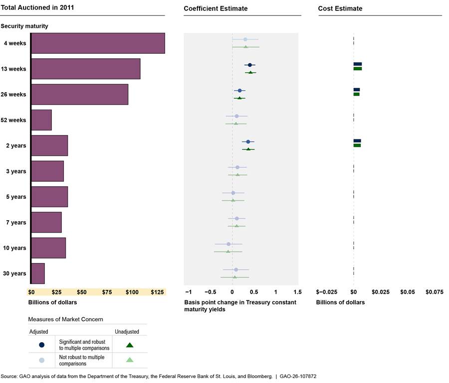
2013 Impasse

For the 2013 impasse, we estimated statistically significant costs associated with 4- and 26-week bills and 3-year notes for both sentiment measures (see fig. 8). The unadjusted sentiment measure also identified small costs associated with the 1- and 2-year notes and cost savings associated with the 13-week bill. We were unable to identify a cointegrated benchmark for the 52-week bill for the adjusted measure because of spillovers identified with that measure.

2015 Impasse

For the 2015 impasse, we estimated statistically significant costs associated with 4- and 26-week bills for both sentiment measures (see fig. 9). We found statistically significant associations with several notes, but none met our multiple comparisons screen. We were unable to identify a cointegrated benchmark for the 30-year bond.

2017 Impasse

For the 2017 impasse, we estimated statistically significant costs associated with 4-week bills for both sentiment measures (see fig. 10). We found statistically significant associations with 26-week bills for one measure, but it did not meet our multiple comparisons screen. We were unable to identify a cointegrated benchmark for notes and bonds with maturities 5 years or longer. Note that the scale of debt issued has increased since 2015, reflecting higher debt levels.

2018 Impasse

For the 2018 impasse, we estimated statistically significant costs associated with 4-week bills for both sentiment measures and 2-year notes for the adjusted measure (see fig. 11). We were unable to identify a cointegrated benchmark for 52-week or 3-year notes or 10- or 30-year bonds.

2021 Impasse

For the combined 2021 impasses, we estimated statistically significant costs associated with 4-week bills for both sentiment measures (see fig. 12). We also estimated modest cost savings associated with the 8-week bills for both sentiment measures. While the yield premium associated with 4-week bills was relatively large, the total cost estimate reflects minimal cost savings due in part to the small number of 4-week bills issued. We were unable to identify a cointegrated benchmark for notes and bonds with 2-, 3-, and 5-year notes or 20-year bonds.

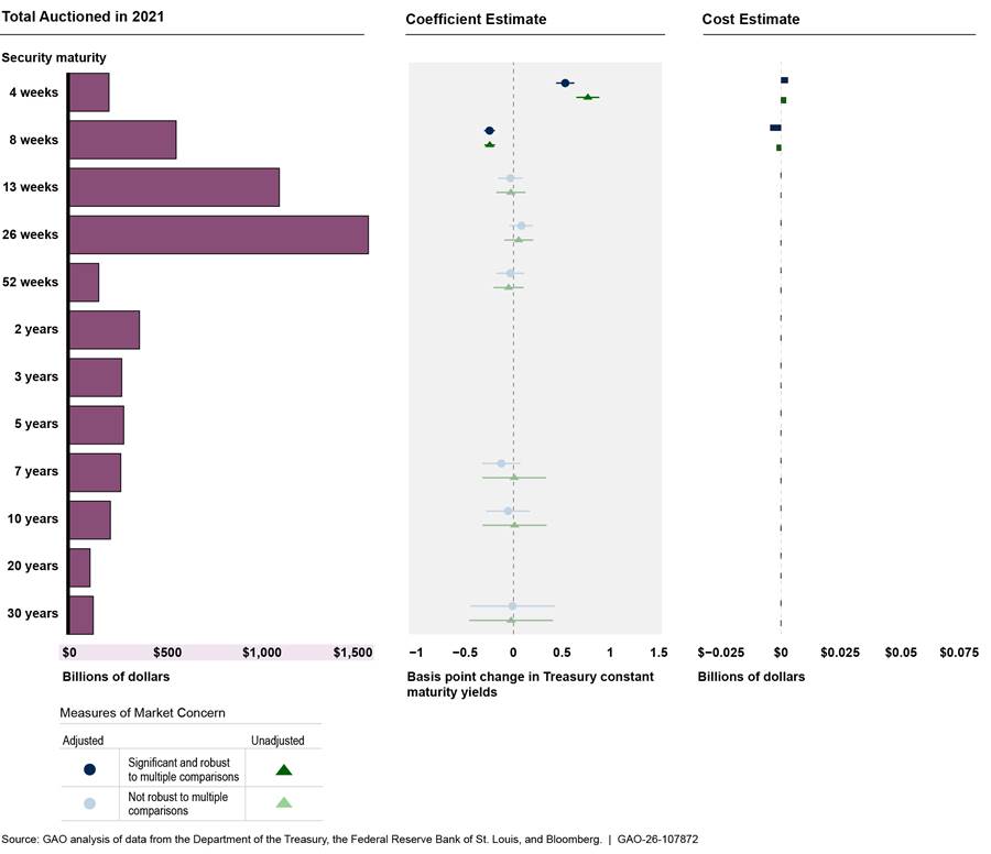
2023 Impasse

For the 2023 impasse, we estimated statistically significant costs associated with 13-week bills for both sentiment measures (see fig. 13). We found statistically significant associations with 4-week bills for one measure and negative statistically significant associations for the other measure that did not meet our multiple comparisons screen. We found a negative statistically significant relationship with 5-year notes for both measures, but only one met our multiple comparisons screen.

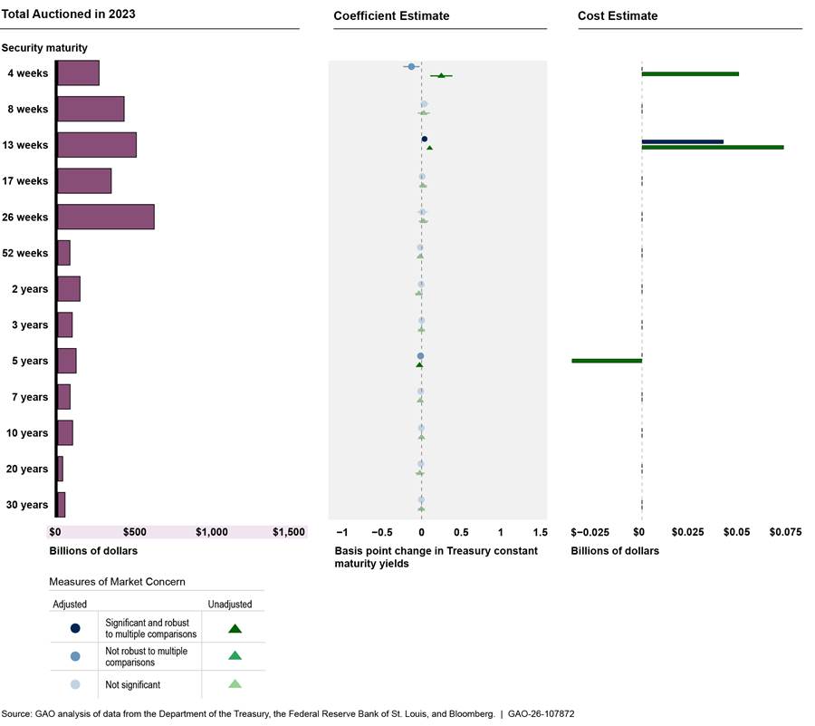
GAO Contacts

Michael E. Clements, clementsm@gao.gov

Michael Hoffman, hoffmanme@gao.gov

James R. McTigue Jr., mctiguej@gao.gov

Staff Acknowledgments

In addition to the contacts named above, Tara Carter (Assistant Director), Emmy Rhine Paule (Analyst in Charge), Michael Bechetti, Abigail Brown, Yiwen (Eva) Cheng, Natalie Duncombe, Brian Harechmak, Christoph Hoashi-Erhardt, Risto Laboski, Jill Lacey, Robert Letzler, Douglas Luo, Daniel Mahoney, Stephen Ruszczyk, Jessica Sandler, and Jennifer Schwartz made key contributions to this report.

GAO’s Mission

The Government Accountability Office, the audit, evaluation, and investigative arm of Congress, exists to support Congress in meeting its constitutional responsibilities and to help improve the performance and accountability of the federal government for the American people. GAO examines the use of public funds; evaluates federal programs and policies; and provides analyses, recommendations, and other assistance to help Congress make informed oversight, policy, and funding decisions. GAO’s commitment to good government is reflected in its core values of accountability, integrity, and reliability.

Obtaining Copies of GAO Reports and Testimony

The fastest and easiest way to obtain copies of GAO documents at no cost is through our website. Each weekday afternoon, GAO posts on its website newly released reports, testimony, and correspondence. You can also subscribe to GAO’s email updates to receive notification of newly posted products.

Order by Phone

The price of each GAO publication reflects GAO’s actual cost of production and distribution and depends on the number of pages in the publication and whether the publication is printed in color or black and white. Pricing and ordering information is posted on GAO’s website, https://www.gao.gov/ordering.htm.

Place orders by calling (202) 512-6000, toll free (866) 801-7077, or
TDD (202) 512-2537.

Orders may be paid for using American Express, Discover Card, MasterCard, Visa, check, or money order. Call for additional information.

Connect with GAO

Connect with GAO on X, LinkedIn, Instagram, and YouTube.
Subscribe to our Email Updates. Listen to our Podcasts.
Visit GAO on the web at https://www.gao.gov.

To Report Fraud, Waste, and Abuse in Federal Programs

Contact FraudNet:

Website: https://www.gao.gov/about/what-gao-does/fraudnet

Automated answering system: (800) 424-5454

Media Relations

Sarah Kaczmarek, Managing Director, Media@gao.gov

Congressional Relations

David A. Powner, Acting Managing Director, CongRel@gao.gov

General Inquiries

https://www.gao.gov/about/contact-us